For an automotive course assignment at RHU in fall 2024, I wrote a simulator for a four-stroke, four-cylinder spark-ignition engine running at 2000 rpm. It covers one full cycle, 720° of crank rotation, and it is built as a chain in which every stage takes the previous one’s output as its input. The geometry gives the volume, the volume gives the pressure, the pressure gives the torque, and the torque sizes the flywheel and the gearbox.
One file of numbers
Every parameter lives in constants.m: link lengths and masses, the engine speed, the timing of intake, compression, combustion, expansion and exhaust in crank degrees, the gas properties, and the flywheel and transmission constants. Each later script loads what the one before it saved, so a change there runs through every result downstream.
The slider-crank
part1.m solves the slider-crank at every crank angle: piston position, velocity and acceleration, the angle of the connecting rod, and the cylinder volume. It does this twice, once with the cylinder axis passing through the crankshaft and once with the two offset by −18 mm, with compression ratios of 9.8 and 10.1. The same pass computes the rod’s angular velocity and acceleration and the accelerations of each part’s centre of mass, which the torque calculation needs later.
A cycle that has to agree with itself
part2.m runs a single-zone thermodynamic cycle over that volume. Compression and expansion are polytropic. Combustion takes 60° around top dead centre: a constant-volume heat addition from the fuel’s heating value gives the temperature at the end of combustion, and a Wiebe function, with a = 5 and m = 2, sets how much of the charge has burned at each angle in between.
The gas exchange is where the cycle loops back on itself. Exhaust blowdown and intake are modelled as compressible flow through a valve orifice, and the gas left over from the exhaust mixes with the fresh charge. That mixture sets the temperature at the start of the next compression, which changes everything after it. So the script runs the cycle again until the temperature at the end of intake matches the one it started compression with.
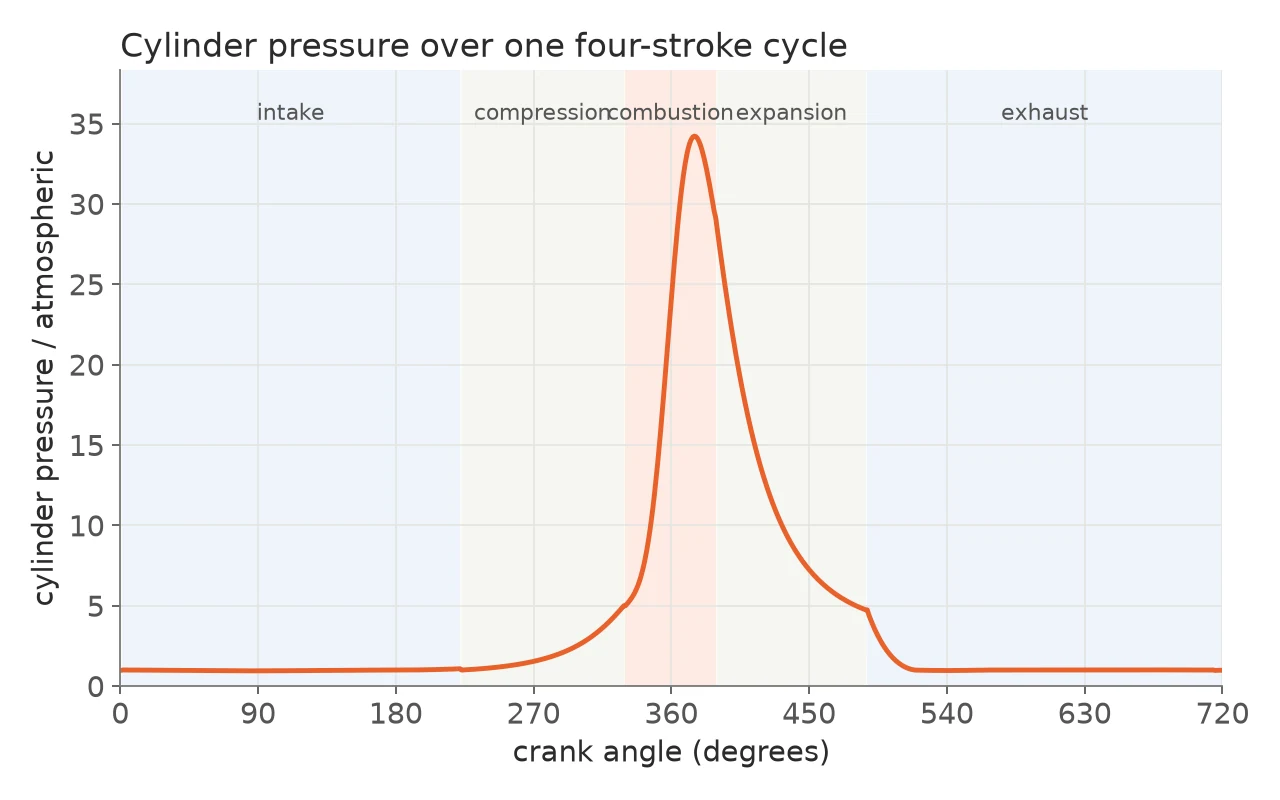
From gas pressure to crank torque
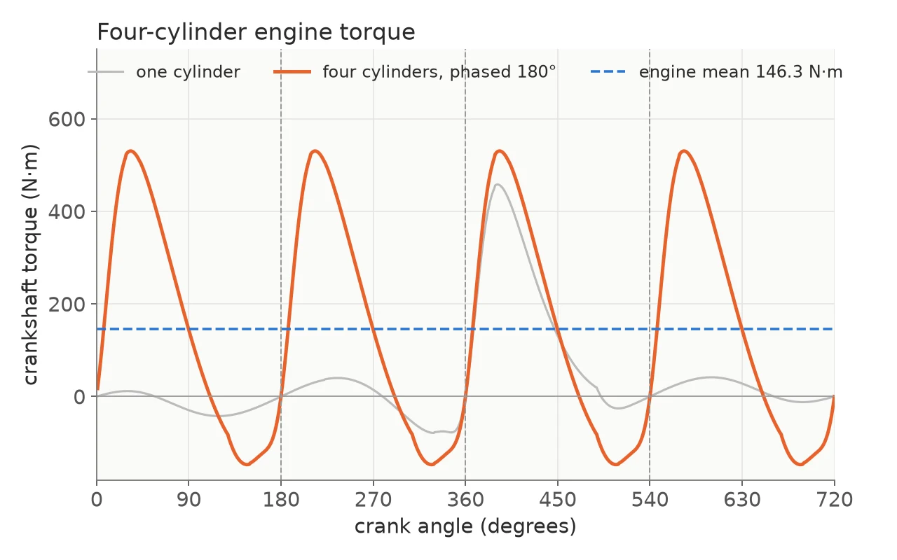
With the pressure known, the torque comes from the forces on the mechanism. At every crank angle the script writes the force and moment balances for the crank, the connecting rod and the piston, including their masses, the rod’s rotational inertia, gravity and the gas force on the piston, as an 8×8 linear system, and solves it for the torque on the crank.
That is one cylinder. The other three are the same curve shifted by 180°, 360° and 540°, and their sum is the torque of the engine.
Flywheel and gearbox
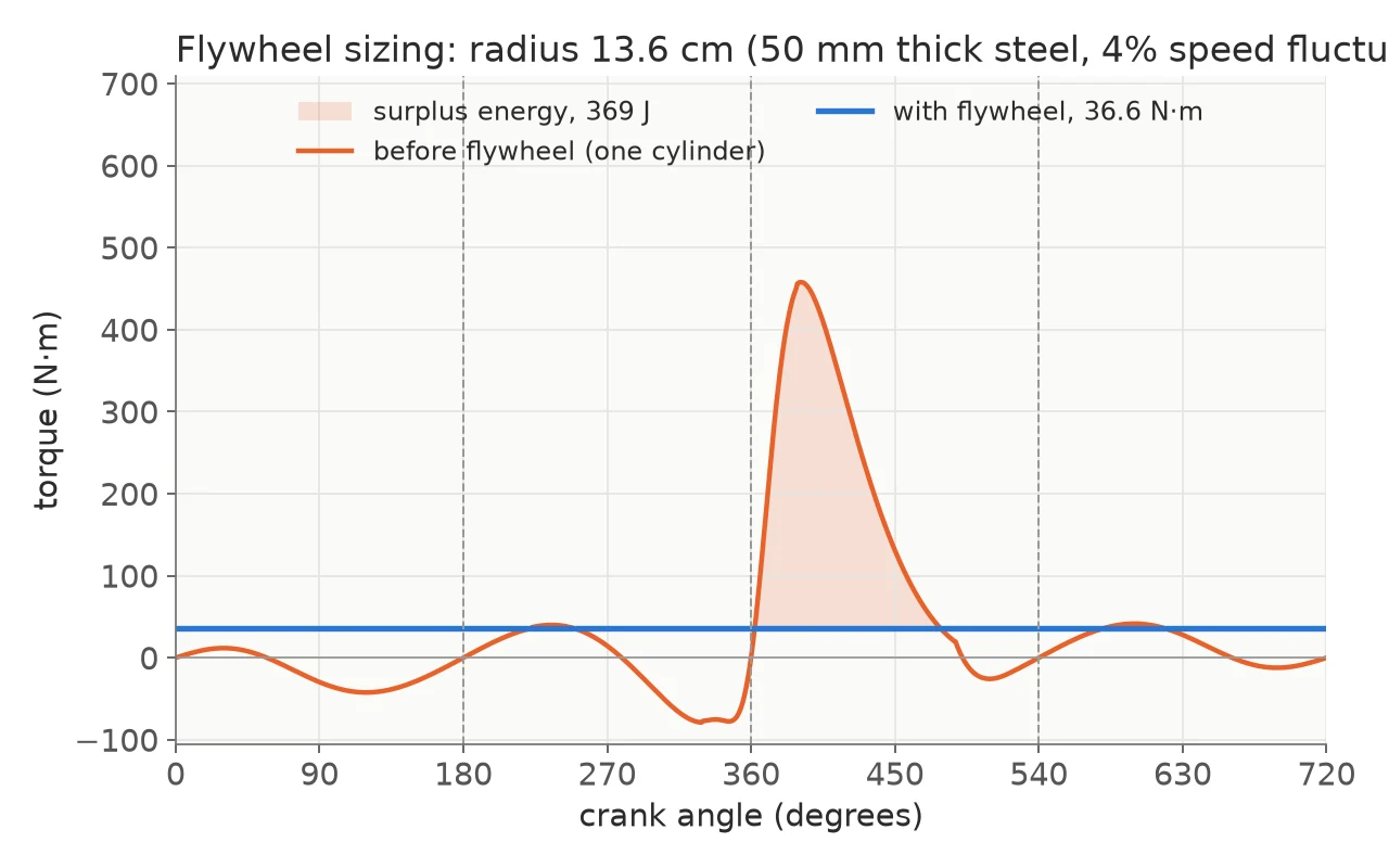
A cylinder’s torque swings above and below its mean over a cycle. The script integrates the energy of that excess between the crossings of the mean and sizes a flywheel to hold the speed fluctuation to a coefficient of 0.04, as a steel disc 50 mm thick; its radius follows from the inertia it needs.
The same run reports the engine’s performance: work per cycle from the pressure–volume loop, indicated and brake power, mean effective pressure and brake mean effective pressure, efficiencies, specific fuel consumption, volumetric efficiency and mean piston speed.
For the engine in the assignment, that comes to about 460 J of work per cylinder per cycle, 30.6 kW of indicated power from four cylinders, and a fuel conversion efficiency of 28 %.
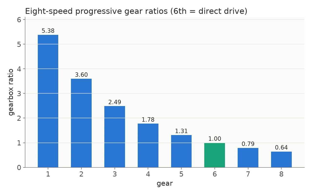
The last step designs an eight-speed gearbox. The top gear is set by a top speed of 245 km/h, the first gear by what it takes to move a 2600 kg vehicle up a 7 % grade while accelerating, and fsolve finds the two factors of a progressive series of ratios between them.
Watching it run
animation.m draws the four slider-cranks moving together and flashes each cylinder as it fires. It makes the phase shift that the torque sum depends on visible.
What it leaves out
These are coursework scripts. Friction is a flat 10 % of indicated power. There is no heat loss to the cylinder walls, no emissions model and no knock. The engine turns at one fixed speed, and the speed-fluctuation curve is an idealised sine between the flywheel’s limits rather than a simulation of the shaft. The mean effective pressures it prints are also about half what they should be, because the displacement constant is smaller than the engine’s swept volume of about 503 cc.